All examples
Google Sheets

Build a sales dashboard in Google Sheets

One 1:39 screen recording, 10 clicks, no script. TurtleScene turned it into everything below. Nothing was edited by hand.

In1:39 recording
Out19
  • 10 videos
  • 1 clickable demo
  • 2 GIFs
  • 2 thumbnails
  • 2 caption tracks
  • 1 help article
  • 1 set of launch posts
The three main outputs

Watch it, click through it, or share the story.

Script, AI voiceover, zooms and a highlight on each step, all generated from the recording. Turn the sound on.

Cut for social · 8 videos

Every shape a feed asks for.

Captions are burned in, in big phrases, so they play muted. The narrated video gets vertical and square cuts that follow every click under a step header, and a 30-second highlight in landscape and 9:16. The story video is laid out again for each shape: vertical and square cuts, and its highlight in landscape and 9:16.

Vertical cut
Reels, Shorts, TikTok · 1:13
Square cut
LinkedIn and X · 1:13
30-second highlight
Emails and landing pages · 0:34
Vertical highlight
Stories and ads · 0:34
Written from the same recording

The docs and the launch copy come with it.

Help article

How to build a sales dashboard in Google Sheets

Create a simple sales dashboard by summarizing your spreadsheet data with a pivot table, then adding a chart and slicer. Follow these steps in order to build the dashboard from your existing dataset.

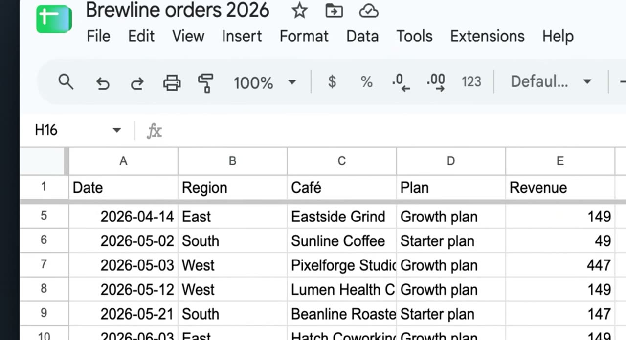
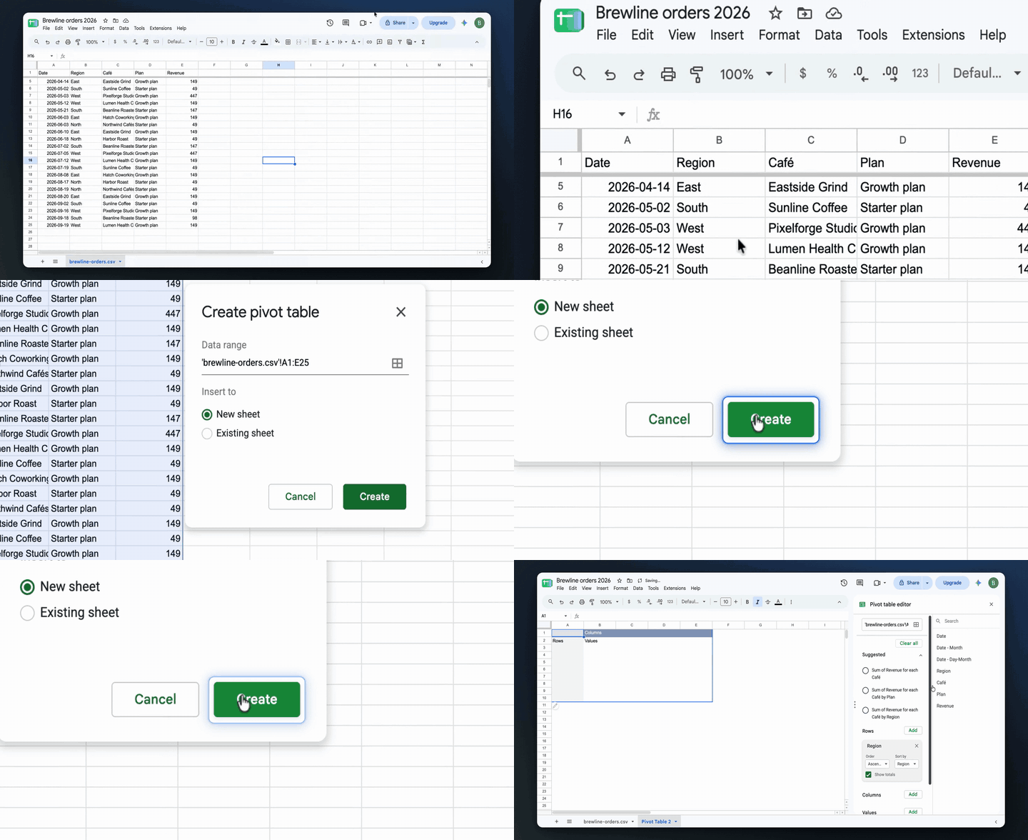
1. Select all data
Select all data

Click the top-left corner cell area of the sheet to highlight the entire dataset. Make sure all rows and columns in your table are selected before you continue.

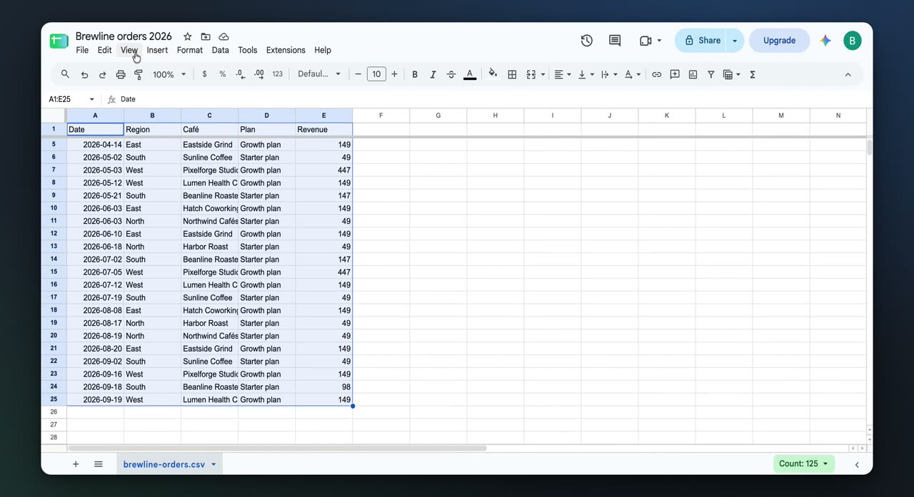
2. Open the Insert menu
Open the Insert menu

With the data still selected, click Insert in the top menu bar. This opens the options for adding something based on the selected data.

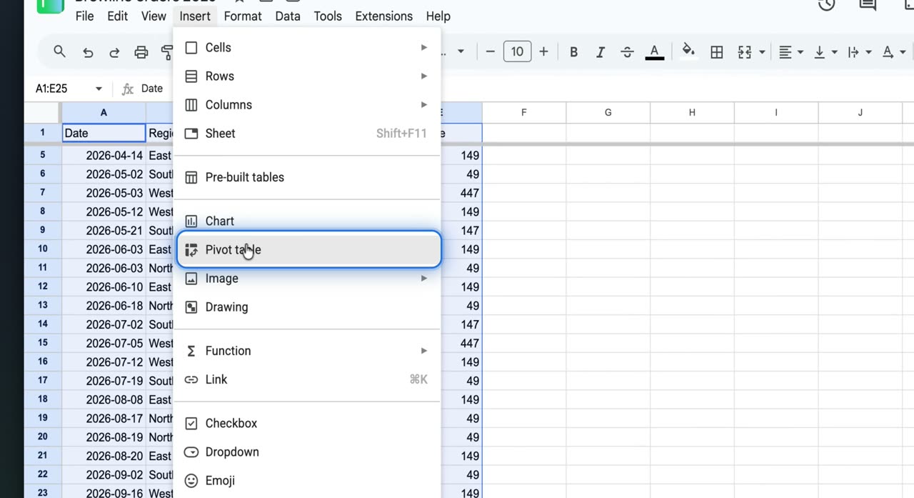
3. Choose Pivot table
Choose Pivot table

In the Insert menu, click Pivot table. This opens the pivot table setup dialog.

4. Create the pivot table
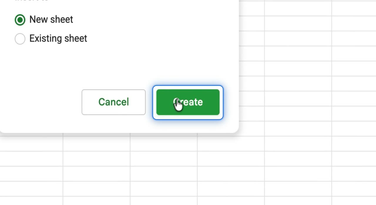
Create the pivot table

Leave New sheet selected, then click Create. Google Sheets adds a new sheet with a pivot table and opens the Pivot table editor.

5. Add a row field
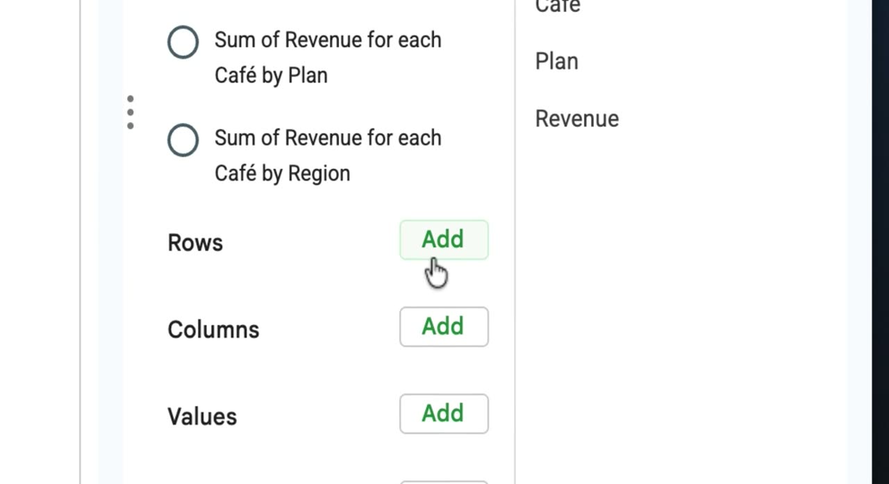
Add a row field

In the Pivot table editor, click Add next to Rows. Choose the field you want to group by, such as Region.

6. Add a values field
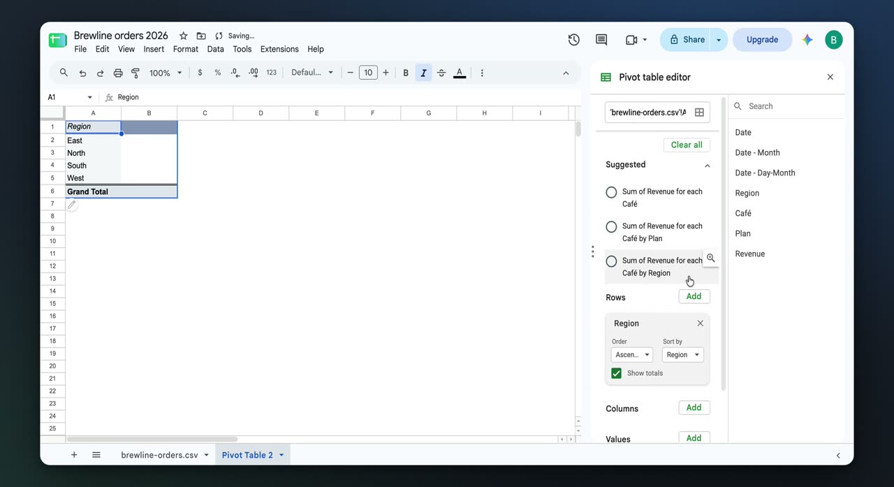
Add a values field

Click Add next to Values in the Pivot table editor. Choose the metric you want to summarize, such as Revenue, so the pivot table shows totals by region.

7. Insert a chart
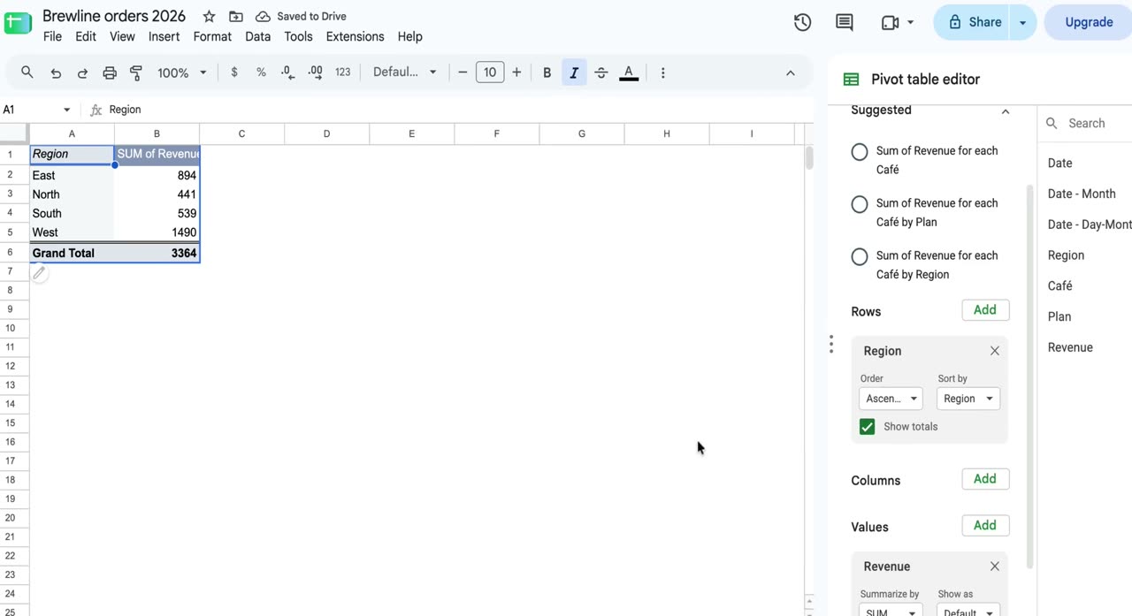
Insert a chart

Open Insert again from the top menu and add a chart based on the pivot table summary. A column chart is created from the pivot table data.

8. Add a slicer
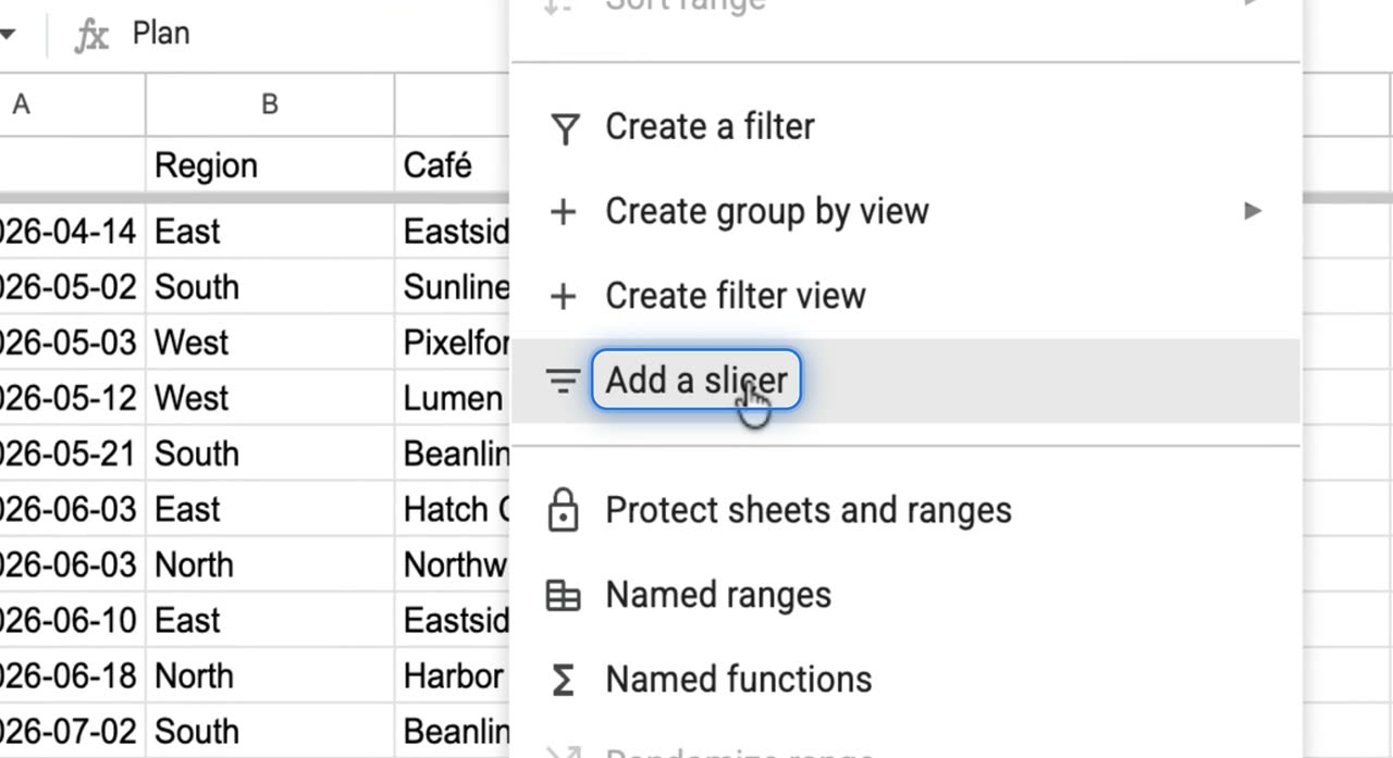
Add a slicer

Open the Data menu and click Add a slicer. This inserts an interactive filter you can use with the dashboard.

9. Set the slicer column
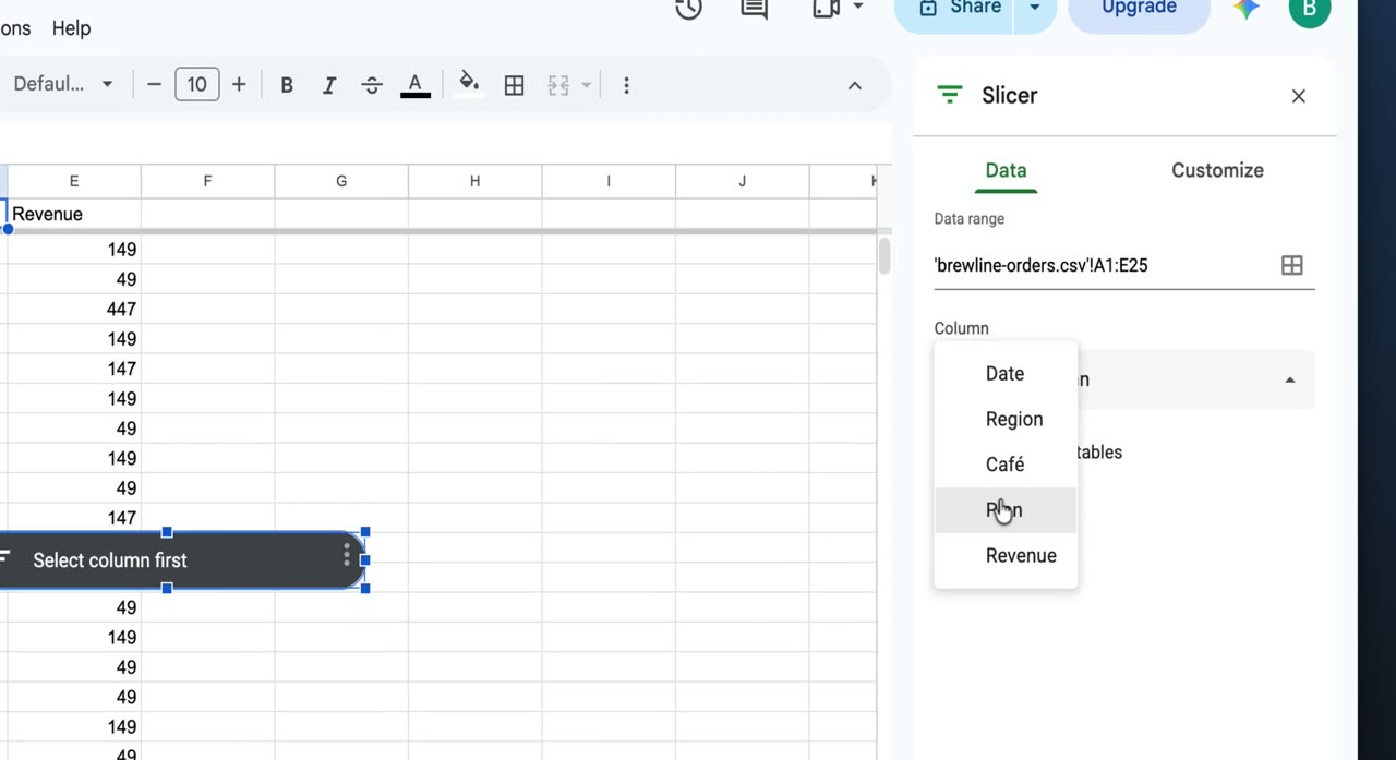
Set the slicer column

In the side panel, choose Plan as the slicer column. This makes the slicer control filtering by plan type.

10. Filter the dashboard
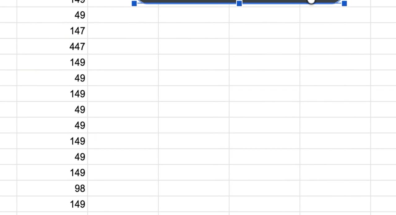
Filter the dashboard

Open the slicer values and clear Growth plan to filter it out. The slicer, pivot table, and chart update together on the sheet.

Your dashboard is now set up, and you can keep adjusting the pivot table, chart, or slicer to explore your sales data.
Launch posts
You
Your company
LinkedIn post · written by TurtleScene

Raw order data rarely tells the full story on its own.

This walkthrough shows how to turn a list of café orders into a simple sales dashboard in Google Sheets using three core steps: summarize, visualize, and filter.

First, create a pivot table from the Insert menu. Add Region as rows and Revenue as values to group sales into something readable.

Next, insert a chart to turn that summary into a bar chart of revenue by region.

Then add a slicer from the Data menu, set it to the Plan column, and choose Growth plan to focus the dashboard on a specific segment.

By the end, you have a clear view of revenue by region, plus a quick way to filter what you see without rebuilding the analysis.

If you’re new to Google Sheets and want a practical first dashboard, this video breaks it down step by step. Watch the video. #GoogleSheets #SalesDashboard #DataAnalysis

You
Your company
X post · written by TurtleScene

Turn raw orders into a simple sales dashboard in Google Sheets.

This quick walkthrough shows how to build a pivot table, add a bar chart, and use a slicer to filter by plan. Watch the video. #GoogleSheets #DataAnalysis

Read the blog post

Build a sales dashboard in Google Sheets with a pivot table, chart, and slicer

Turn raw orders into a clearer view

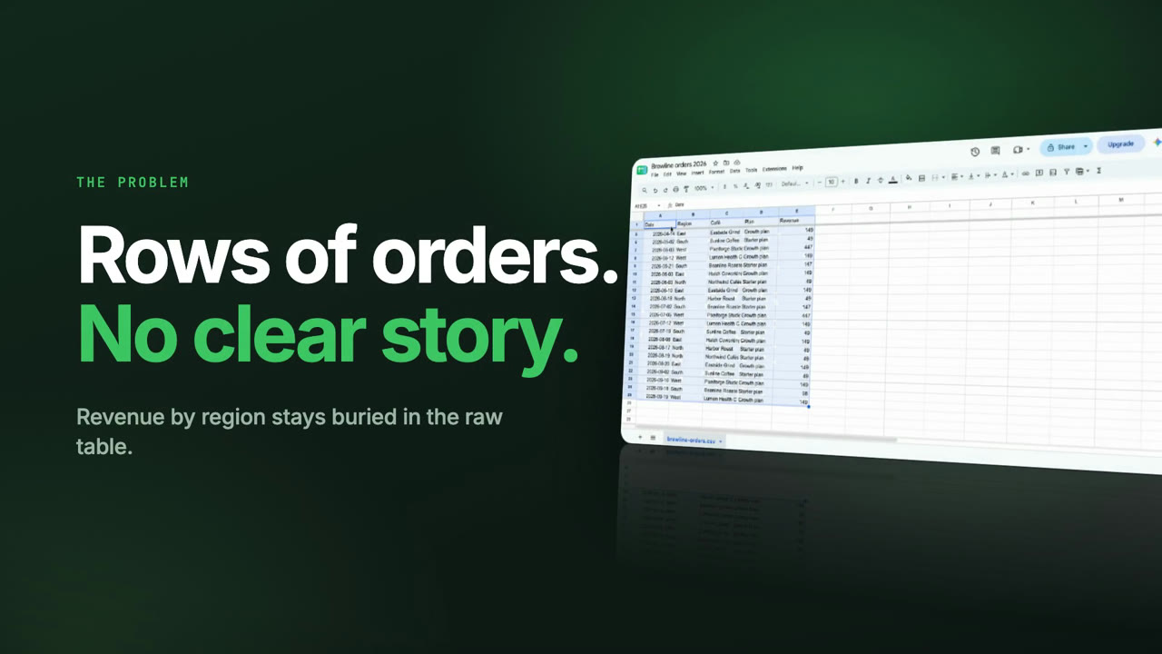
A spreadsheet full of orders can be hard to read at a glance. Row after row of transactions shows activity, but not much insight until the data is summarized.

This video walks through a simple way to build a sales dashboard in Google Sheets using a pivot table, a chart, and a slicer. It’s a practical setup for first-time users who want to move from raw data to a more useful view.

What the video covers

The walkthrough starts with a list of café orders in Google Sheets. From there, it shows how to summarize revenue by region with a pivot table.

The steps are straightforward:

  • Open the Insert menu
  • Choose Pivot table and click Create
  • Add Region as rows
  • Add Revenue as values

That creates a simple summary table that groups revenue by region.

Make the summary visual

Once the pivot table is in place, the next step is to make it easier to scan.

The video shows how to return to the Insert menu and add a chart. Google Sheets then plots revenue for each region as a bar chart, giving the dashboard a visual layer that’s easier to interpret quickly.

This is especially useful when you want to compare regions without reading through every number in the table.

Add a filter with a slicer

To make the dashboard more flexible, the final step is adding a slicer.

Using the Data menu, the video adds a slicer, sets its column to Plan, and selects Growth plan. That filter narrows the view so the pivot table and chart focus on a specific segment of the data.

The result is a simple dashboard: revenue by region, displayed in both table and chart form, with a slicer to refine the view.

A simple first dashboard to try

If you’re getting started with Google Sheets, this is a useful example of how to summarize, visualize, and filter data without overcomplicating the process.

Watch the video and try the same flow with your own data: pivot, chart, and slice in Google Sheets.

Captions · narrated video
  1. 00:00Here's how to build
  2. 00:01a sales dashboard in Google Sheets.
  3. 00:04Select the top-left corner
  4. 00:06so the full dataset is highlighted.
  5. 00:10With the table selected, open the Insert
  6. 00:12menu to add something based on this data,
  7. 00:15and choose Insert from the top toolbar.
  8. 00:18From Insert, choose Pivot table
  9. 00:21to open setup.
  10. 00:23Keep New sheet selected,
  11. 00:25then create the pivot table.
  12. 00:29In the Pivot table editor,
  13. 00:30add a field under Rows.
  14. 00:33Region is already in Rows,
  15. 00:35and the table updates on the left.
  16. 00:37Add a field under Values
  17. 00:38so the pivot can summarize a metric.
  18. 00:42The pivot now shows Region and Revenue.
  19. 00:45Open Insert again so we can add
  20. 00:47a chart based on this summary table.
  21. 00:50A column chart appears,
  22. 00:52then the view returns to the source sheet.
  23. 00:56Under Data, add a slicer for filtering.
  24. 01:00Set the slicer column
  25. 01:02to Plan in the side panel.
  26. 01:05Open the Plan slicer values
  27. 01:07and clear Growth plan so the chart filters
  28. 01:10to the remaining option.
  29. 01:13The slicer, pivot table,
  30. 01:15and chart stay visible on the sheet.
  31. 01:19The sheet now shows a pivot chart
  32. 01:21with a Plan slicer.
Captions · story video
  1. 00:00Here's how to turn raw café orders
  2. 00:02into a simple sales dashboard
  3. 00:04in Google Sheets.
  4. 00:07Line after line of orders shows
  5. 00:09very little until you summarize it.
  6. 00:12From the Insert menu, choose Pivot table
  7. 00:15and click Create. Then add Region
  8. 00:18as rows and Revenue as values.
  9. 00:22Open Insert again and add a chart.
  10. 00:25Google Sheets plots revenue
  11. 00:26for each region as a bar chart.
  12. 00:29Next, open the Data menu and add
  13. 00:32a slicer, set its column to Plan,
  14. 00:34then pick Growth plan to filter.
  15. 00:38The result: a pivot table
  16. 00:39and chart of revenue by region,
  17. 00:42with a slicer to focus the view.
  18. 00:45Try it with your own data: pivot,
  19. 00:47chart, and slice in Google Sheets.
For previews and link cards

GIFs and thumbnails, from both videos.

GIF · narrated video
GIF · narrated videoChangelogs, READMEs, emails
GIF · story video
GIF · story videoChangelogs, READMEs, emails
Thumbnail · narrated video
Thumbnail · narrated videoYouTube and link previews
Thumbnail · story video
Thumbnail · story videoYouTube and link previews

Independent tutorials we recorded ourselves. Google Sheets is a trademark of their owners; TurtleScene is not affiliated with or endorsed by them.

Your next product demo is one recording away

Record a flow on the free plan and watch it come back narrated, clickable and on-brand in a few minutes.

  • No credit card
  • 2 free recordings a month
  • Cancel any time